Why do bell curves appear everywhere?

Why do most probability graphs show a bell curve?

As you suspect, there is a natural tendency for distributions to be bell-shaped.

There are some distributions that are not bell-shaped at all. For example, the outcome of a roll of one fair die is a discrete uniform distribution:

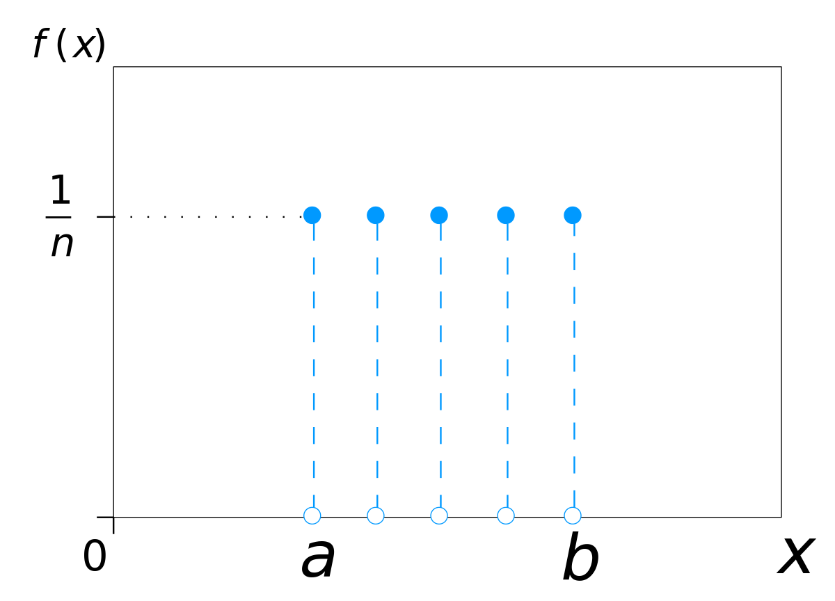
By IkamusumeFan - Own work This drawing was created with LibreOffice Draw, CC BY-SA 3.0, Link

The roll of one die is a pretty simple process. What about the sum of two dice? The Wizard of Odds illustrates:

Starting to look a little like a bell, right? What about the totals of three, or four dice? Wolfram MathWorld provides a nice illustration:

You can see where this is headed. Nature is full of complex processes. How tall are you? Well, it depends on genetics, nutrition, exercise, injuries, bone loss, and so many more things. The central limit theorem shows (see symplectomorphic's comment below) that when adding the sum of a large number of things together, the resulting distribution is not just any bell-looking curve, but specifically the normal distribution. Or for things with multiplicative combination, the log-normal distribution.

Why does this happen? mathreadler's answer hints it has to do with convolving distributions. The probability density function of a single die is a rectangular function (technically discrete, but let's pretend it's continuous). The sum of two rolls together is then the convolution of two rectangular functions.

By Convolution_of_box_signal_with_itself.gif: Brian Amberg derivative work: Tinos (talk) - Convolution_of_box_signal_with_itself.gif, CC BY-SA 3.0, Link

Notice how the result (the black triangle) looks like the case of two dice above. If then convolve this triangle with another rectangle, you get three dice. The more times you do this, the closer the result gets to a normal distribution.

The probability density function of the normal distribution is a Gaussian function, which have some elegant properties:

• A Gaussian convolved with a Gaussian is another Gaussian.
• The product of two Gaussians is a Gaussian.
• The Fourier transform of a Gaussian is a Gaussian.

From this you might intuitively see as things converge towards normal distributions, they "want" to stay as normal distributions since their "Gaussianess" is preserved under many operations.

Of course not everything is so simple as a single die roll, nor as complex as the determination of the height of a human. So there are a large number of distributions that look like a bell, but on careful examination aren't the normal distribution. Some of them exist in nature, and some find application as mathematical tools for some purpose. Looking through Wikipedia's list of probability distributions you can see bell-like shapes are quite common, even if they aren't exactly the normal distribution.

But if you combine these two things:

• The central limit theorem means the normal distribution is common, and
• many distributions look like bells but aren't the normal distribution,

you might conclude most probability graphs show a bell curve.

The convolution of two functions is at least as nice as the nicest of the two (often even nicer), and the sum of two independent distributions has a density which is the convolution of their density functions. So as they convolve more and more when we add them up they become nicer and the gaussian function is the nicest in the world!

I think it is important to distinguish between the general bell shaped curves that not have to be normal and the normal distribution. For the later, the key notion, as already mentioned and elaborated, is the Central Limit Theorem. Namely, if some slightly technical conditions are satisfied then sample averages and sums converge (weakly) to the normal distribution. However, $(1)$ not every bell shaped curve is normal and $(2)$ not everything that we assume that is normal is indeed normal. As already was mentioned in the comments - a lot of biological variables are definitely not normal (like heights and weights of humans) however they are bell shaped and can be approximated with very high precision with the Gaussian distribution. Same relation you can encounter with the Exponential distribution as a model for life duration of machine or something like this - they are definitely not really exponential as the machine cannot "live" forever.

As such, maybe a better model will be truncated distributions. E.g., heights maybe well described by two side truncated normal distribution. But what are the problems in this case? $(1)$ If the truncation values (parameters) are unknown, you have to estimate them, and $(2)$ besides it may introduce much more complexity to your calculations. So the basic questions in statistical modelling (IMHO) is not "whether this or that variable follows the normal distribution" albeit whether the Gaussian random variable can give us a good approximation of its distribution. Let us take the heights of healthy adult males in Scandinavia for example. A good model for their heights distribution will probably be $N(187, 10)$, but more accurate model will be the same Normal distribution but truncated at $5$ standard deviations above and below the mean, i.e., setting the support to be $[137, 237]$. Your gain in precision in estimating probabilities is absolutely neglectable as this truncation adds less than $0.001$ to the "mass" of the bell at $[137, 237]$. Same logic applies to the machine's life duration example. A truncation at $\tau$ that is far away from the expected value will give you correction term that is $1/P(X<\tau) = 1/(1-e^{-\lambda x})$, and it equals almost $1$, thus you have no practical gain from this.

Another issue that was already mentioned, is that asymptotic normality is not a universal truth. N.N. Taleb called the Gaussian distribution "the great intellectual fraud", where, to the best of my understanding, he meant that in finance the exponential decay ("thin" tails) is very uncommon feature. Namely, you can take Cauchy's distribution for example, it also has a bell shaped form, however due to relatively "fat" tails, it does not have a finite mean. This distribution will serve as a bad approximation of the heights of humans because negative heights or "gigantically" large values (let us say, over $4$ meters) are biologically impossible. Hence, a fat tail distribution that puts non-neglectable weights on extreme values will be improper mathematical modelling of such variable (height). While, in revenues it may be vice versa - assuming normality is the same as assuming neglectable probabilities for very large gains or losses, that - as we all know - maybe simply wrong.

To sum it up, it seems that symmetry and general "bell" shape is indeed prevalent in the real world distributions. However, strict normality as described by $$ f_{X}(x) = \frac{1}{\sqrt{2 \pi \sigma^2}}\exp\left\{-\frac{(x-\mu)^2}{2\sigma^2}\right\}, $$
is mostly just an approximation of the actual distribution. More accurate models that are still "bell" shaped may be better in calculating various parameters, however the little gain from the more precise model usually don't worth the higher complexity that it introduces. Hence, the regular normal distribution remains in many cases not only a good approximation but also a very convenient one. Finally, it is worth to mention that are some "domains" like finance where the bell shaped distributions are mostly non-normal ones, and assuming normality in this case may be wrong.